Anatomy of a Bond Movie

It’s January 2021. It’s almost a year into the pandemic in the UK, we’re in lockdown, and we’re finding ways to stay busy and entertained. Over the last few weeks my young man took a fascination with Bond Movies, and we’ve end ended up watching all the PG ones at a rate of almost 1 per night.

This starkly revealed the formula for a Bond Movie, as they very clearly all follow a pattern of similar events and constructs.

I decided to capture it on paper. It fits pretty well with the 15 or so we’ve seen so far.

Anatomy of a Bond Movie: most of the movies seem to follow a generic formula

2 years of car driving data - analysis (including stage 1 remap)

I love driving and I love data. So why not combine the two? Well, I have.

At the time of writing I’ve had what-I-still-think-of-as-my-new-car for just shy of two years since new and every trip has been (intentionally) logged. What’s more, for the latter 7.5 months or so it has been running with a stage 1 map.

I initially started collecting my journey data because I was keen to see whether anything changed about the car as it was “run in”. (It did; but not for the reasons I expected). Data is acquired quite easily because it is all logged automatically by the car to its Skoda portal, although it only gives aggregate (average) data per trip. But that’s plenty to get started with.

I pull the data down every so often in excel and convert to CSV. I then point Tableau at these CSV files in order to build the visualisations. Because tableau can refresh and union multiple files automatically the process is fairly painless (despite Skoda conspiring to make it more awkward after their portal update) .

I learnt plenty of things along the way which I didn’t really consider in the first instance. But that’s the beauty of Tableau, because it’s so easy to slice, dice and re-visualise the data, that you can look at it in new ways without any heavy lifting.

So, the very first thing I wanted to look at

Long term economy

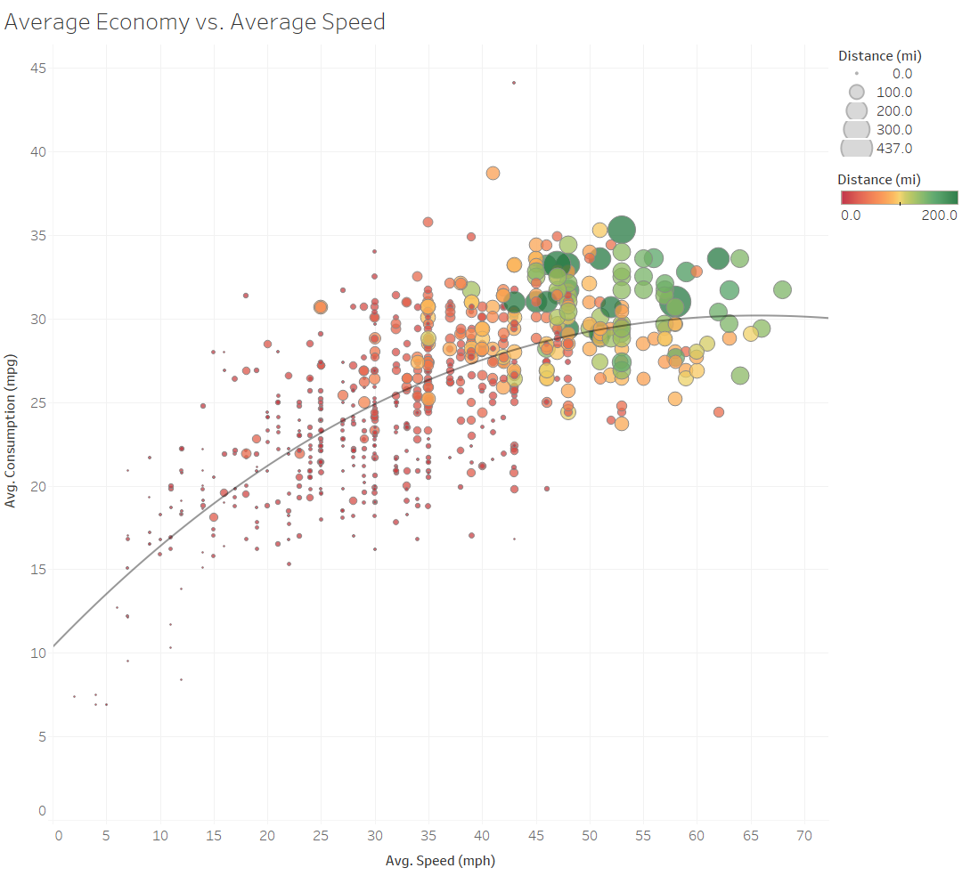
The simplest analysis of long term economy is simply to plot average trip speed against average economy returned. This pretty much comes out as we’d expect: that here is a sweet spot for economy once you’re up to a consistent cruising speed. Bear in mind, of course, this is not “instantaneous” economy at a given speed, but whole-trip average. For this reason I’ve plotted the size of the trip as the size of the circles and unsurprisingly we can see longer trips (green) towards both the upper end of average speed and average consumption.

Average trip economy vs. Average trip speed

The variation in results is, of course, due to many factors: weather, traffic, road condition, state of the vehicle, vehicle load and my driving style. I am by no means a “hyper miler” but some journeys I do drive a bit more economically. On the other hand, I’m not afraid to overtake in order to make safe and reasonable progress - so I tend to use a varied spectrum of the car’s capabilities.

There are probably several choices for the “best fit” regression curve. A straight line clearly doesn’t cut it as economy does not keep on increasing as the car goes faster. In the end I have used a polynomial of degree 3.

Perhaps what is surprising (to me) about this result, as it’s not something I’ve thought much about before, is how poor the economy is for short trips of low speed: trips to the shops and the like.